Hypothesis Testing: One-way ANOVA
What is a One-way ANOVA?
A one-way ANOVA is an inferential technique to assess two competing hypotheses about the population means across k samples. Specifically, one-way ANOVA tests whether the k population means are equal. If there is significant evidence that the population means are different, we want to conduct post hoc testing to investigate where the means are different.
One-way ANOVA evaluates the equality of k population means based on observed data under the following conditions.
1. The observations are representative of the population of interest and independent. The samples are mutually independent.
2. The observations within each sample are normally distributed.
3. The variances within each sample have equal variance (note that Welch's ANOVA does not require this assumption).
The one-way ANOVA F statistic compares the observed data with what we expect under the null hypothesis, which states all of the population means are equal. The resulting p-value tells us how likely observing the evidence we have for the alternative hypothesis or more when the null hypothesis is true. If the p-value is less than the specified significance level (e.g., less than 0.05), we reject the null hypothesis in favor of the alternate hypothesis. In that case, the one-way ANOVA test indicates that we have significant evidence that at least one population means is different. Otherwise, we fail to reject the null hypothesis, indicating we do not have significant evidence that at least one population means is different.
If the one-way ANOVA test result is significant, we can conduct post hoc tests to investigate which means differ. The post hoc test for the traditional one-way ANOVA test is Tukey's Honest Significant difference; it corrects for multiple simultaneous inferences. The corresponding test for Welch's ANOVA for data with unequal variances across samples is the Games-Howell test.
How to use this app?
Step 1: To use this app, go to the 'Dataset and Hypothesis' tab and upload your .csv type dataset, or select a sample dataset.
Step 2: Next, you must select the type of ANOVA (traditional one-way ANOVA or Welch's ANOVA for unequal variances across samples).
Step 3: You can check the assumptions provided in the 'Assumptions' tab. We recommend assessing assumptions visually using the provided graphical summary and confirming using the numerical summaries. The app will provide results for a Fligner-Killeen Test assessing common variance across samples and Shapiro-Wilkes (n ≤ 5000) or Kolmogorov-Smirnov (n > 5000) tests for normality. While these tests might be helpful, they can be rather sensitive for small sample sizes leading us to detect minuscule transgressions.
Step 4: You can check the result of the ANOVA procedure (test statistics, decision making, and test visualization) in the 'Hypothesis Test' tab.
Step 5 (Optional): If the ANOVA procedure produces a significant result, you can view the results of the appropriate post hoc procedures in the 'Post Hoc' tab.
Contact us
Please contact us if you have any questions at datascience@colgate.edu.
Example 1
Within the one-way ANOVA app, we provide the penguin data that includes measurements for penguin species inhabiting islands in Palmer Archipelago and made available through the palmerpenguins library for R (Gorman et al., 2014). Suppose researchers aimed to evaluate whether species of penguins (Adelie, Chinstrap, and Gentoo) have differing mean flipper lengths (mm). This is a classic example of a scenario requiring the one-way ANOVA test framework.
Here, we have three samples of observations (the species) and a continuous attribute (flipper length). We will use the one-way ANOVA procedure to evaluate whether the data support the claim that at least one species has a different population mean flipper length.
First, we load the one-way ANOVA app. Second, we click 'Sample Data' to load the penguin data. Once the data are loaded, we select the variable (flipper_length_mm) and the sample (species). The data summary provides our first look at the data.
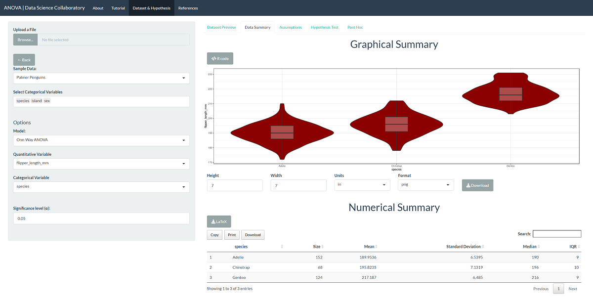
The first step of conducting the one-way ANOVA procedure requires us to evaluate the assumptions. When we click 'Assumptions', the data are plotted for interpretation.
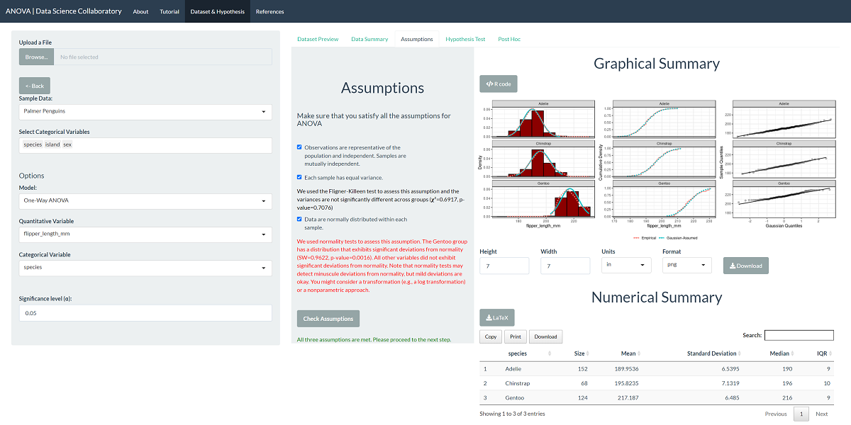
This plot shows that the data are roughly normally distributed as the densities are symmetric and bell-shaped. The variances are similar as the spread of the distributions are almost identical. We note that evaluating whether the observations are representative of the population of interest and independent is more challenging. These data were collected from many penguin nests across three different islands in Palmer Archipelago, meaning the data are likely to be representative. We trust that the researchers collected data in a way that made the observations near independent.
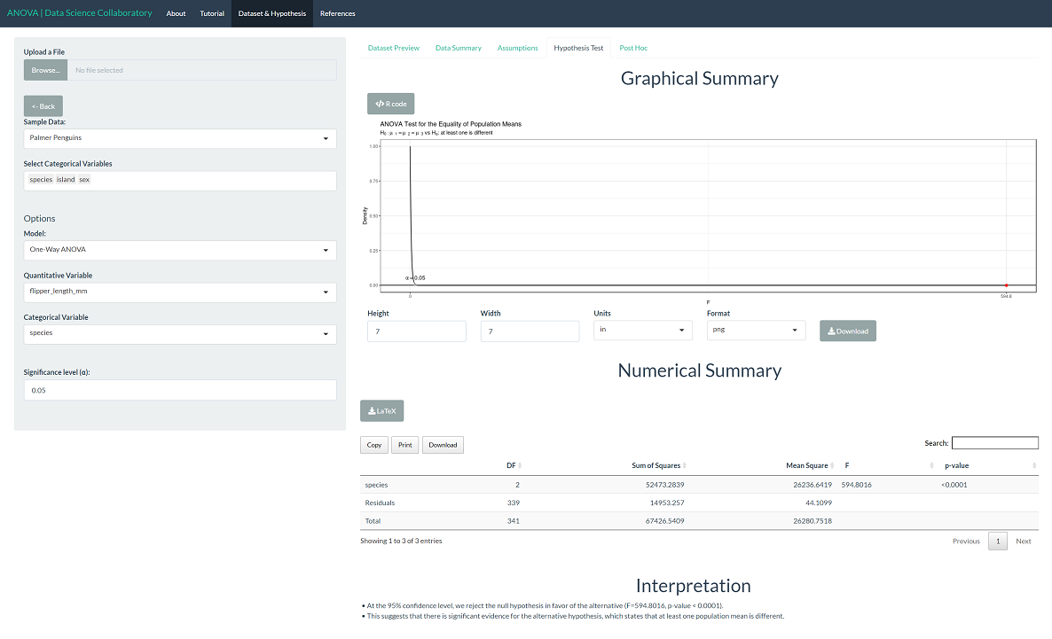
The 'Hypothesis Test' tab shows the result of the one-way ANOVA procedure. As we might expect after checking the assumptions, there is significant evidence that the population mean flipper lengths (mm) differ across species (F=594.8016, p<0.0001). This tells us that at least one population mean is different but not which population means or in what direction.
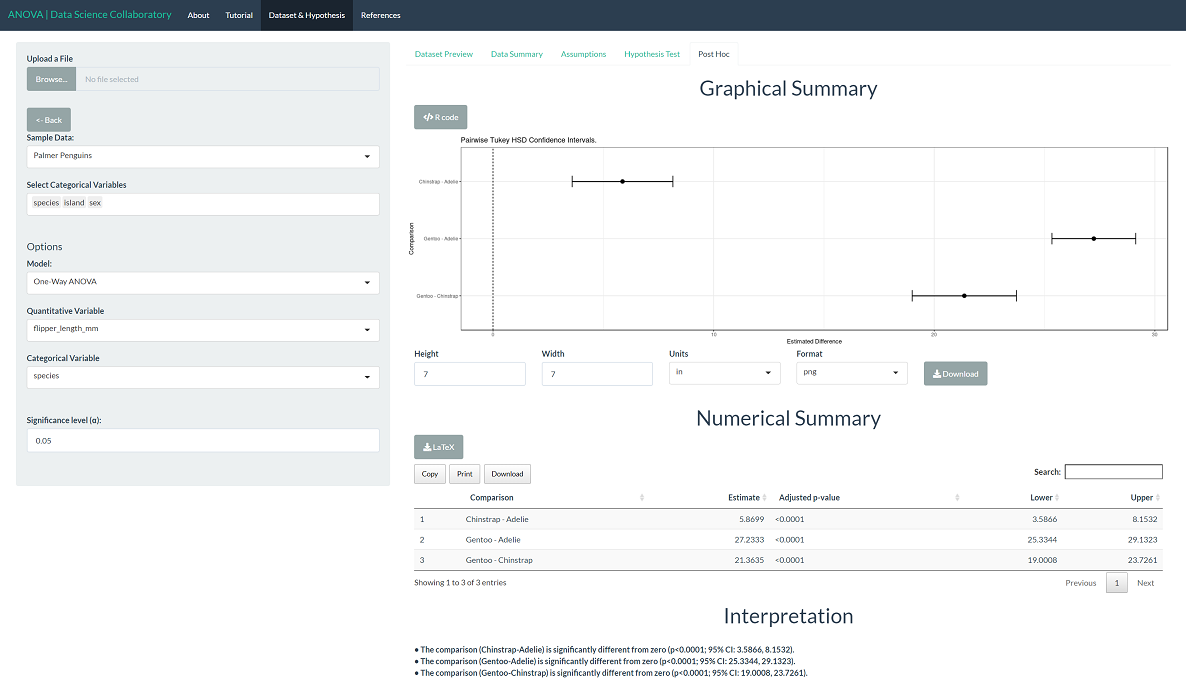
To evaluate differences among the populations, click 'Post Hoc'. All differences are statistically significant, with p-values less than 0.0001. This is not all that surprising. As observed in the assumptions plot, Gentoo penguins have visibly different flipper lengths (mm). While Chinstrap and Adelie are closer in flipper length (mm), they are still significantly different based on our observations.
Gorman KB, Williams TD, Fraser WR (2014) Ecological Sexual Dimorphism and Environmental Variability within a Community of Antarctic Penguins (Genus Pygoscelis). PLoS ONE 9(3): e90081. doi:10.1371/journal.pone.0090081
Example 2
Within the one-way ANOVA app, we provide the MFAP4 data that includes measurements for Hepatitis C patients collected by the German network of Excellence for Viral Hepatitis and studied by Bracht et al. (2016). These researchers aimed to evaluate whether the human microfibrillar-associated protein 4 (MFAP4, U/ml) varies across the fibrosis stages (0, 1, 2, 3, 4) in hepatitis C patients. The researchers can use the one-way ANOVA testing framework to evaluate MFAP4 as a biomarker for disease stages.
Here, we have five samples of observations (the fibrosis stages) and a continuous attribute (MFAP4 U/ml). We will use the one-way ANOVA procedure to evaluate whether the data support the claim that the MFAP4 levels vary across fibrosis stages; i.e., at least one fibrosis stage has a different population mean MFAP U/ml.
First, we load the one-way ANOVA app. Second, we click 'Sample Data' to load the MFAP4 data. Once the data are loaded, we select the variable (MFAP4) and the sample (Fibrosis.Stage). The data summary provides our first look at the data.
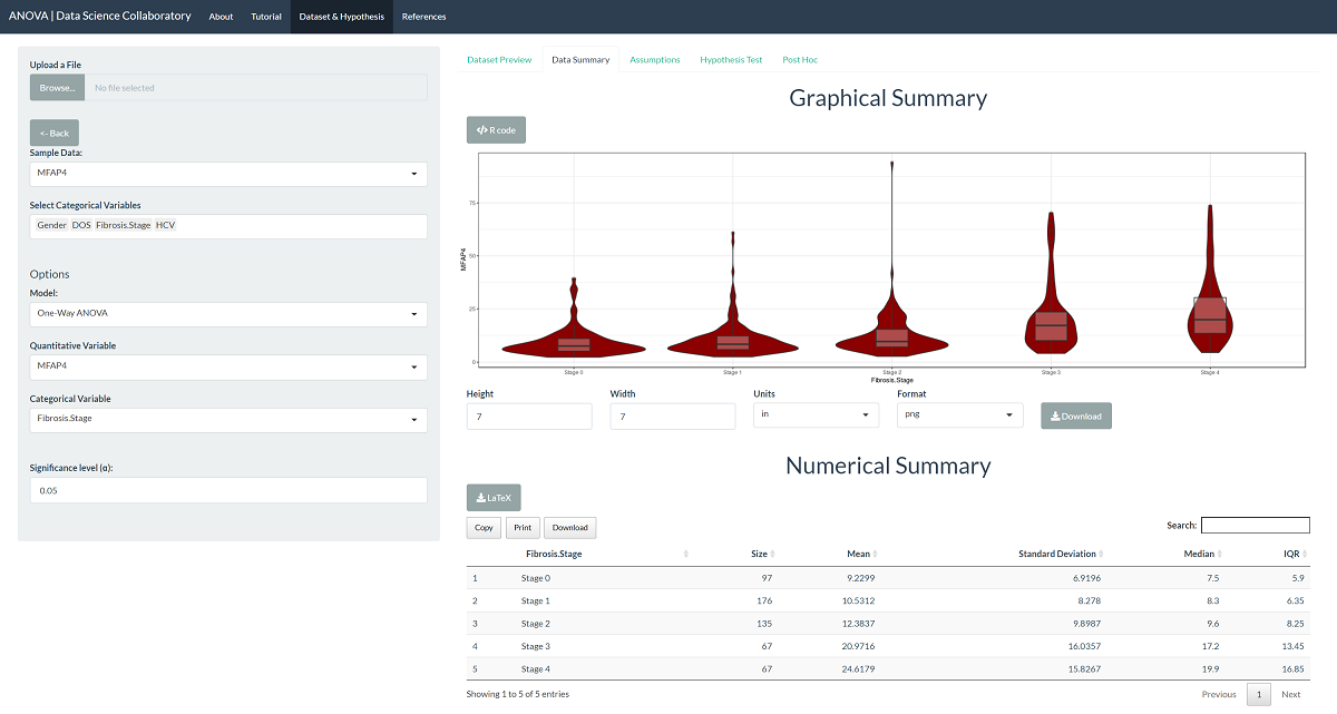
The first step of conducting the one-way ANOVA procedure requires us to evaluate the assumptions. When we click 'Assumptions', the data are plotted for interpretation.
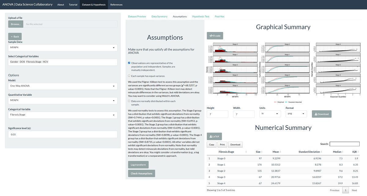
At this point, we observed the data are heavily skewed, and the variances differ. We note that evaluating whether the observations are representative of the population of interest and independent is more challenging. In their paper, Bracht et al. (2016) tell us these data were collected at different sites using a protocol meant to reduce bias, meaning the data are likely to be representative. We trust that the researchers collected data in a way that made the observations near independent.
Based on this information, we have several choices. We can (1) use a transformation (e.g., the log) or (2) use a non-parametric test like a Mood's Median Test or the Kruskal-Wallis Test for mean ranks. We note that Bracht et al. (2016) use a log base-2 transformation for their data, and the transformed data are in the sample data. We will select the variable (log2.MFAP4) and the samples (Fibrosis.Stage), then we can reassess the assumptions in this setting.
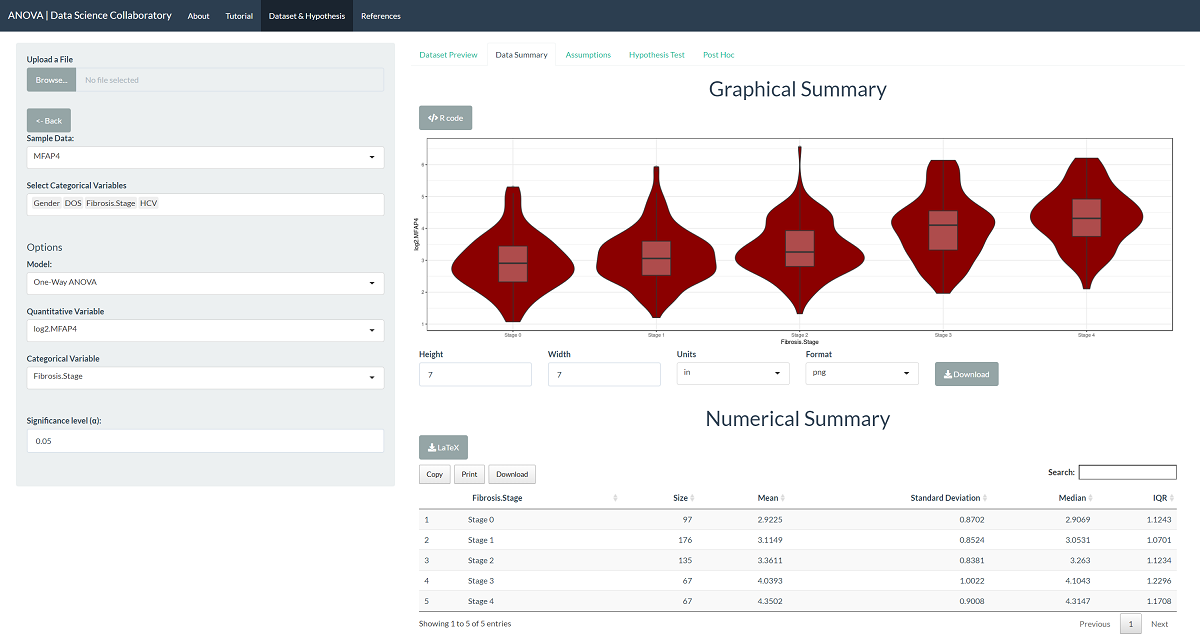
The data summary provides our first look at the data. The violin plot shows that the transformed data are closer to meeting our normality and equal variance assumptions. When we click 'Assumptions', the plots confirm that the data probably fit the assumptions of the one-way ANOVA model.
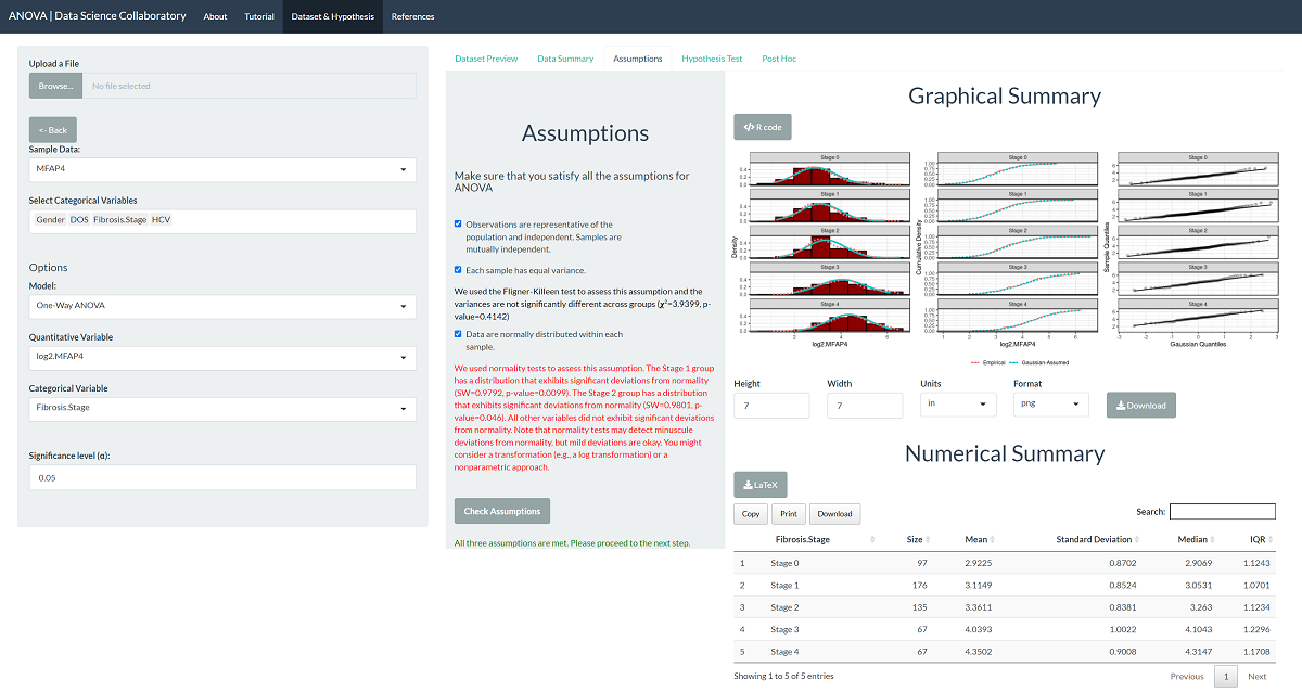
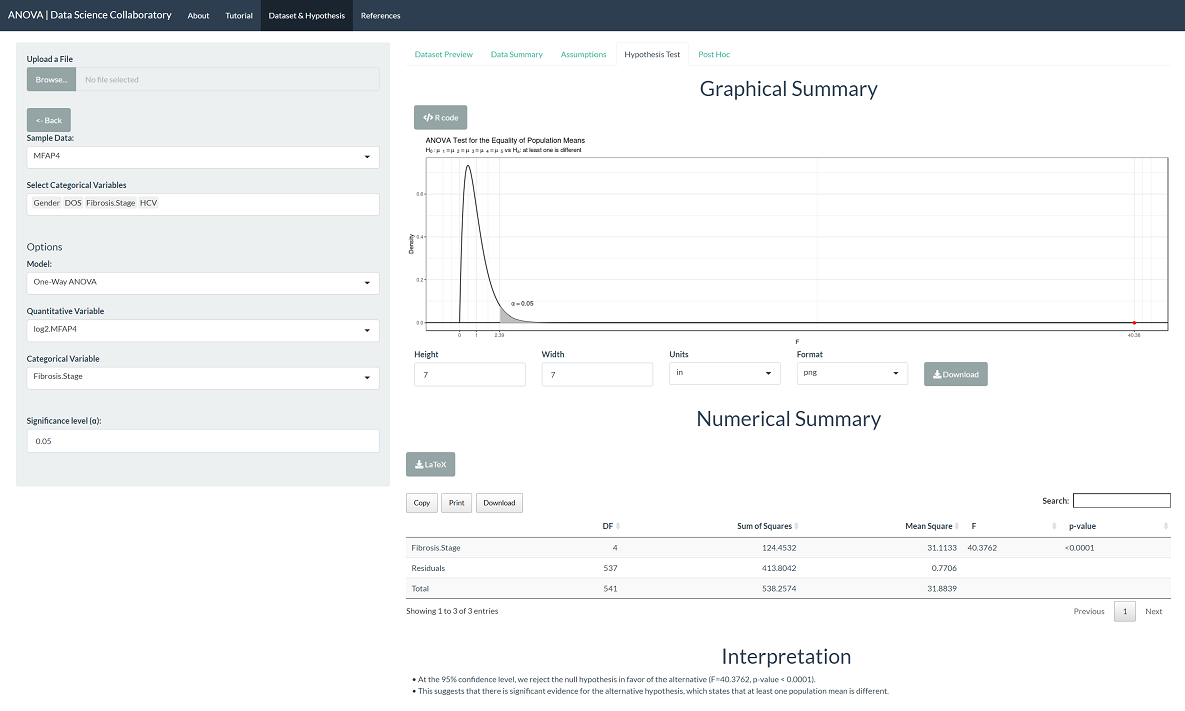
The 'Hypothesis Test' tab shows the result of the one-way ANOVA procedure. As we might expect after checking the assumptions, there is significant evidence that the population mean MFAP4 U/ml levels differ across fibrosis stages (F=40.38, p<0.0001). This tells us that at least one population mean is different but not which population mean(s) or in what direction.
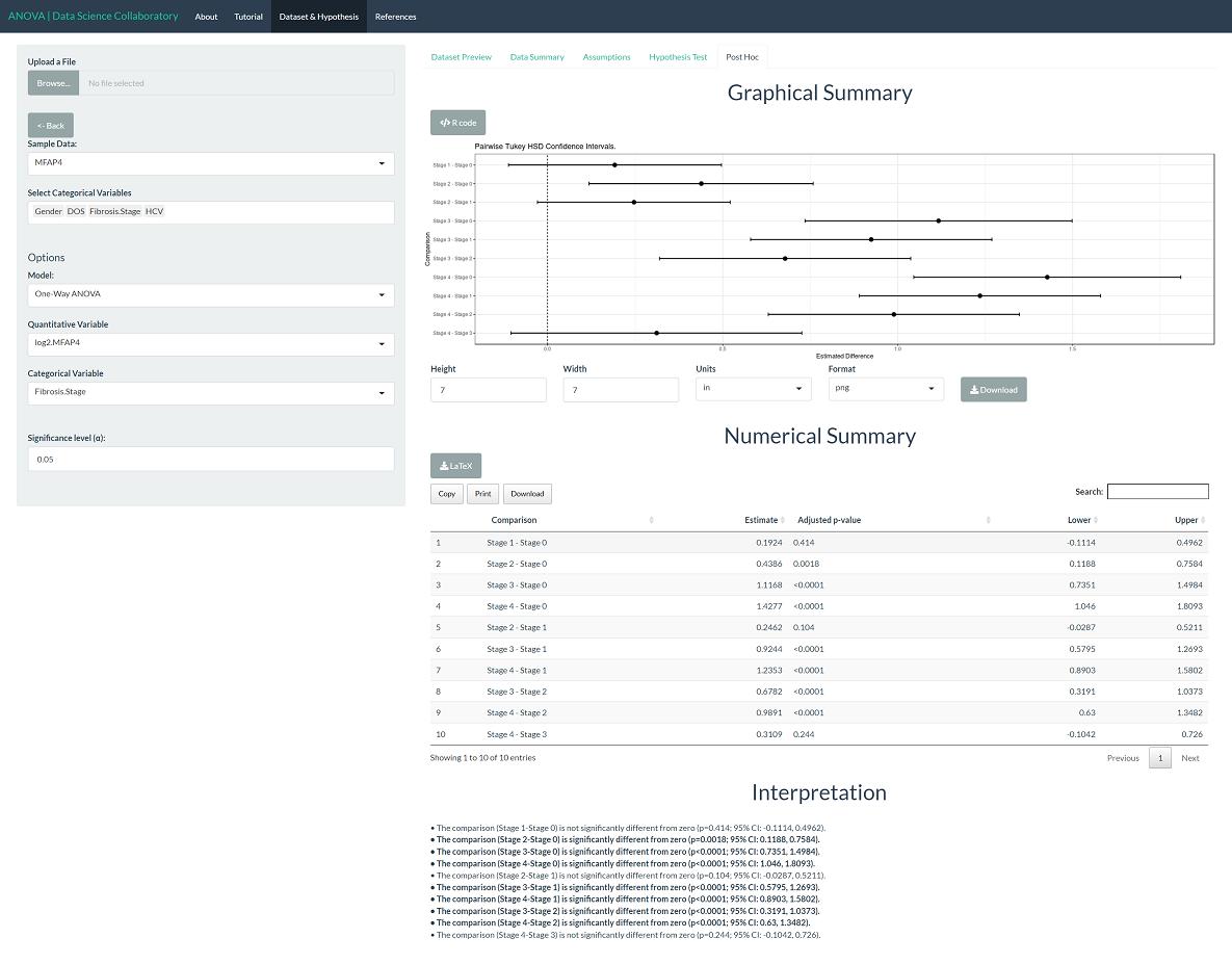
To evaluate differences among the populations, click 'Post Hoc'. We see that stage 0 is different from stages 2-4; stage 1 is different from stages 3-4; stage 2 is different from stages 0, 3-4; stage 3 is different from stages 0-2; and stage 4 is different from stages 0-2. That is, one-way ANOVA creates groupings (0-1), (1-2), and (3-4). Bracht et al. (2016) suggest that MFAP4 is a promising biomarker for the assessment of no to moderate hepatic fibrosis stages (0-2) from patients with severe fibrosis and cirrhosis (3-4).
Bracht, T., Molleken, C., Ahrens, M., Poschmann, G., Schlosser, A., Eisenacher, M., ... & Sitek, B. (2016). Evaluation of the biomarker candidate MFAP4 for non-invasive assessment of hepatic fibrosis in hepatitis C patients. Journal of Translational Medicine, 14(1), 1-9.
Example 3
Within the one-way ANOVA app, we provide U.S. News and World Report's College Data that includes measurements for many U.S. Colleges from the 1995 issue of U.S. News and World Report and made available through the ISLR library in R (James et al., 2017). Suppose we aimed to evaluate whether alumni donate at different rates at private and public colleges and universities. This is a question we can use the one-way ANOVA test framework to answer, noting that a two-sample t-test is a special case of one-way ANOVA.
Here, we have two samples of observations (private/public) and a discrete attribute (percent of alumni who donate). We will use the one-way ANOVA procedure to evaluate whether the data support the claim that there is a difference in the mean percent of alumni who donate across types of colleges and universities.
First, we load the one-way ANOVA app. Second, we click 'Sample Data' to load the U.S. News College data. Once the data are loaded, we select the variable (perc.alumni) and the samples (private). The data summary provides our first look at the data.
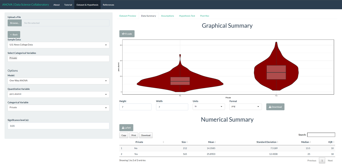
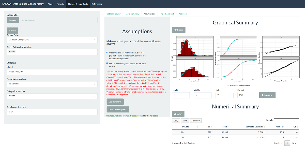
The first step of conducting the one-way ANOVA procedure requires us to evaluate the assumptions. When we click 'Assumptions', the data are plotted for interpretation.
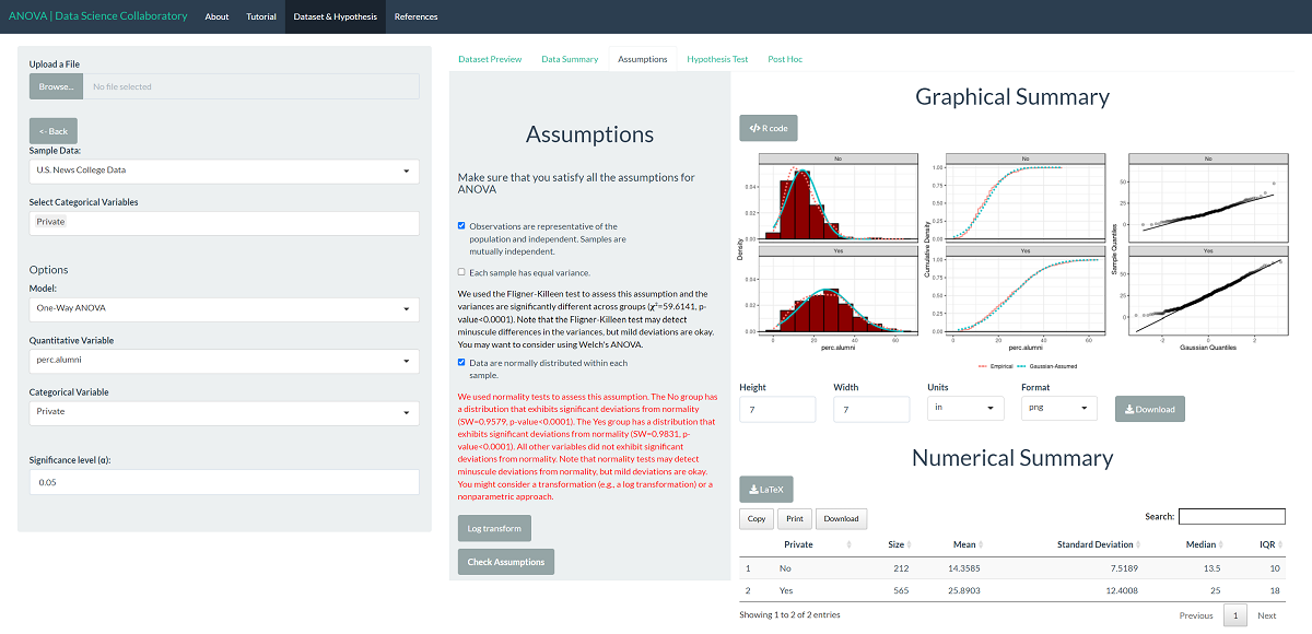
This plot shows that the data are roughly normally distributed as the densities are roughly symmetric and bell-shaped. Still, the variances are somewhat different as the spread is much larger for private institutions. We note that evaluating whether the observations are representative of the population of interest and independent is more challenging. We won't get into how U.S. News conducts its ratings, but it has been heavily scrutinized in the media. For demonstration purposes, we will proceed assuming that the data are representative. The data may be representative, but we'd have to do more digging.
When it comes to the unequal variance assumption, we can circumvent it by switching to Welch's ANOVA for data with unequal variances across samples. Since Welch's ANOVA only assumes that the data are normal and representative, we can proceed with the test.
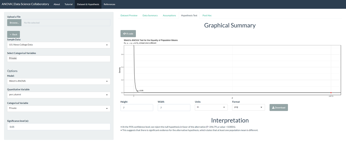
The 'Hypothesis Test' tab shows the result of Welch's ANOVA procedure. As we might expect after checking the assumptions, there is significant evidence that the population mean percentage of alumni that donates differs across institution types (F=246.79, p-value < 0.0001). This tells us that at least one population mean is different, and, of course, we know private is different than public, but not in which direction.
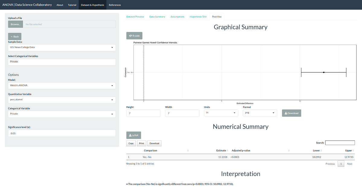
To evaluate differences among the populations, click 'Post Hoc'. The difference is statistically significant, with a p-value less than 0.0001, such that private schools see higher rates of donation among alumni. This is not all that surprising. As observed in the assumptions plot, private institutions have visibly different donation rates among alumni.
Gareth James, Daniela Witten, Trevor Hastie and Rob Tibshirani (2017). ISLR: Data for an Introduction to Statistical Learning with Applications in R. R package version 1.2. https://CRAN.R-project.org/package=ISLR